Allocating Minutes in the NBA
For this project I took a look at the 2016-17 Miami Heat roster and I wanted to create a mathematical model to calculate the best way to divide up (allocate) minutes of playing time. To do this I first analyzed team data from the NBA's 2016-17 Season to see what typically comprises a win. This was done through regression analysis. I used that information to develop theories on what team stat totals should be targeted when trying to win a game. These theories I applied to the construction of a mathematical model that used the rates that the players on the Miami Heat output each statistic and allocated minutes in a way that maximized points while keeping other stats above or below the bounds I included. These bounds I determined from the trends found in team data.
On basketball-reference.com I went through the 2016-17 NBA Season and gathered the Game Logs for each team into an Excel document. This is by team per game data resulting in (30 teams)*(82 games) = (2460 observations). The purpose of these observations is to identify trends in the statistical composition of the different outcomes. I deleted the Opponent columns because that data is already accounted for in other observations and is redundant. Games that went beyond 48 minutes would inflate my data so I eliminated the 70 games (140 observations) that went into overtime. I created a binary variable W. I created the variable PTD. Below is a small subset of my data and a description of my variables.


I ran a regression of these statistics on W and PTD separately. Below are the models followed by the regression output for W and then PTD.


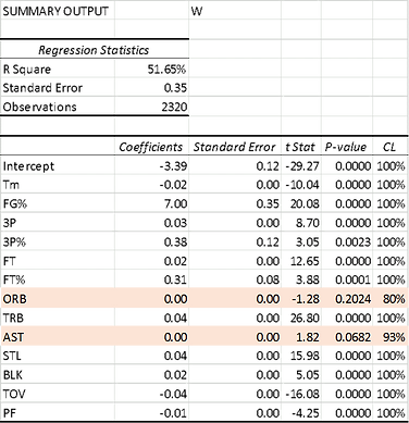
I excluded Opp from the regression because Tm along with Opp explain 100% of PTD. Due to the nature of regression I couldn’t include for example: 3P, 3PA, & 3P%. Thus I left out FGA, 3PA, & FTA. I had issues with FG so it was removed as well. I later realized that FG could be calculated when Tm, 3P, and FT are known so the four of these variables cannot all be included in a model. At the 95% CL ORB doesn’t have a statistically significant impact on outcome in either case so it won’t be included in my model. AST don’t impact the variable W and PF don’t impact PTD. I won’t be including PF in my model because I think that its correlation with W is reverse causation. Often times at the end of a basketball game when the outcome has nearly been determined, the losing team resorts to fouling the winning team. This is why I argue that losing leads to fouling not the other way around. AST will remain in my model but will have less weight.
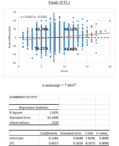
All other stats will appear in my model as either the variable I'm optimizing or as a constraint. To determine where they appear I ran individual regressions for each stat with PTD. The R Square shows how dependent the outcome is on that stat and therefore how important it should be in my model. I also created scatter plots to observe correlations and calculate the threshold where the expected outcome switches. The percentages that appear on the graphs describe what proportion of teams won vs lost that were above or below the threshold of the x-intercept. For example as shown in the first graph; 71.17% of teams that scored more than 105.0556 points won while teams who scored less than 105.0556 points won only 30.10% of the time. Below are two examples

Next is a summary of the R Square values and x-intercepts for each of the variables.

Referring to the table above, I’ll be using Tm as the dependent variable in my objective function. Following that is the order that I’ll be adding them into the model as constraints. I won’t be including all of the constraints initially because there probably wouldn’t be a feasible solution. I’ll proceed through adding one stat at a time, see if there’s a feasible solution, and then determine if the trade-offs were worth it. Notice they’re in order of descending R Square with the exception of AST which I gave a little penalty for not having a statistically significant impact on W.
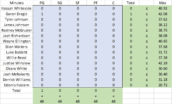
The objective function will have minutes as independent variables. Minutes will need to be split into 75 different variables, 5 for each player where each one is for a certain position.

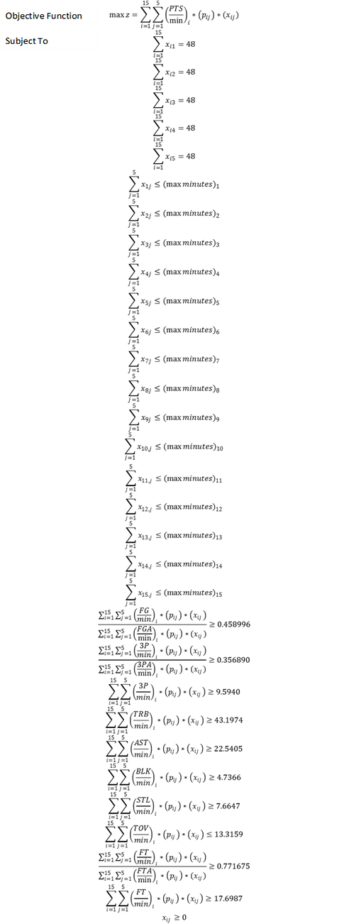
The natural constraints for this matrix is that 48 minutes exactly must be allocated to each position and each player needs a limit on the number of minutes they can play. This gives me the following objective function and some constraints.
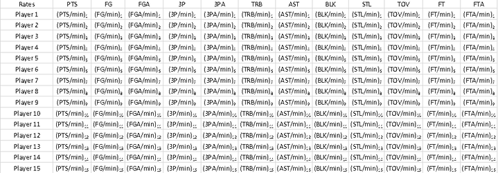
The rest of the constraints will be the team output for each stat being at least (or at most for TOV) the x-intercept. I use the x-intercept because this is where the expected outcome changes from a loss to a win. Defining the unknown rate coefficients by the next table I get the rest of my constraints. The last constraint says that no player can be assigned negative minutes.
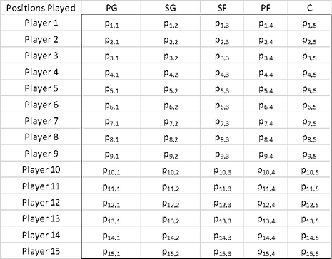
(pij) in the objective function and constraints represents whether the player can play the position or not. This will be a 1 or a 0 which will be multiplied by their rates resulting in no production if they’re playing out of position. The matrix of positions played looks like the following.
The next step is to apply the model to an NBA roster. To pick the team I only considered teams that played the minimum 15 players in the 2016-17 season. I didn’t want to use a team that differed throughout the year. In those cases the players rates are a combination of production in different circumstances.
So for the 2016-17 Miami Heat roster specifically I needed to collect the max minutes each player played in a game this season. Also per minute rates for each player for each stat and what positions they can play. I got per minute rates by dividing per 36 minute stats found on basketball-reference.com by 36. This means that I assumed stat productions are linear functions of minutes which is not a perfect assumption.


Notice I don’t include FG%, 3P%, or FT% in this table. This is because the percentages aren’t directly a function of minutes. If I calculated the expected percentages for each player I couldn’t easily convert that into the team percentages that make up my constraints. The way around this as displayed in the formulas for the constraints is to divide total team FG, 3P, and FT by total team FGA, 3PA, and FTA respectively. A consequence to this is that the model is no longer a linear program. Solver can no longer solve this, I’ll need to instead use Excel’s GRG Nonlinear method to evaluate.
The max minutes I’ll display in the basic ‘feasible’ solution. The basic feasible solution gives Excel a starting point to work with. This isn’t really a feasible solution because not enough minutes are at each position. Notice I put 1 minute into Goran Dragic to start. I did this because if it started out with no FGA, FTA, or 3PA the percentages would be undefined and it would not be able to move forward.
To get these max minutes for each player I used each players game log data from the 2016-17 season on basketball-reference.com. I sorted it by minutes and then eliminated from consideration all of the games that went into overtime. For example here’s the top 5 games in terms of minutes played for Goran Dragic.

Though the degree I'm about to receive is Actuarial Mathematics I don't know that I'll end up going into the Actuary career. My education has been a combination of mathematics, economics, and finance. I believe that the skills I've obtained qualify me for all sorts of work pertaining to business mathematics. In the past I've done regressions (data analysis) and mathematical models but I had never combined the two. That was the purpose of this project.
Data Analysis
Model
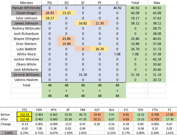
Iteration 9
Constraints: Minutes, FG%, 3P%, 3P, TRB, BLK, TOV, FT
Above is my final solution. Along the way something I did was I multiplied the changes in stat totals by the coefficient from the regression with W to see if the chance of winning increased or decreased to decide if the constraint added was beneficial. In some cases it was not, that's why Assists, Steals, and Free Throw Percentage weren't included as constraints in the end. PS: A logit model is something I’ll consider for future projects.
To see if my results aligned with current perceptions I made the following table. I looked at team rankings of minutes played and salaries to see where each player stands compared to my result. I adjusted everyone's actual minutes per game to total 48 minutes (It didn’t before because it doesn’t include games where they played zero minutes).

Compared to some general perceptions it seems that my model overvalues Derrick Williams, Luke Babbitt, and Wayne Ellington and undervalues Justise Winslow, Dion Waiters, and Josh Richardson. I think that a lot of current opinions are based solely on point production. My first iteration that was only points looked more like the real minute distribution. The argument for my model is that young players (Winslow & Richardson) got playing time regardless of performance so they could develop. In a one-game must-win situation though it's not unrealistic to suggest that they don't play. The argument could also be made that maybe Waiters is overrated because of his turnovers and shooting percentages where Ellington and Babbitt may be better alternatives. Derrick Williams is a very curious case because my model maxed out his minutes throughout, yet he got cut from the team mid-season and is the only one who wasn't on a roster going into the 2017-18 season.
References
(https://www.basketball-reference.com/teams/BOS/2017/gamelog/)
(https://www.basketball-reference.com/teams/BOS/2017_games.html)
(https://www.basketball-reference.com/teams/MIA/2017.html)
(https://www.basketball-reference.com/players/d/dragigo01/gamelog/2017)